Linkedin Excel Assessment test questions with answers of 2021

linked excel assessment test questions with answers

Microsoft Excel is one of the programs in Microsoft Office. Excel is a spreadsheet program which is developed for Windows, Mac, IOS, etc. An Excel spreadsheet is filled with a number of columns and rows. 
Microsoft Excel helps to perform data determination and data analysis. Microsoft Excel is a well known and powerful program used by business functions and companies from all over the world. The demand for Excel expert employees is increasing day by day. This is why job seekers need to take Excel skill assessment test to improve their Excel skills.
𝓠1: What is usually on an Excel Assessment?

Excel Assessment is a kind of assessment test where you can justify your Excel skill efficiency. It is very helpful to know skill level, improvement level, performance level. Excel Assessment test can be varied by Basic level, Middle level and Advance level, depending on job position.

But there is no specific level in Linkedin Excel Assessment. Here comes the question about all kinds of features in Microsoft Excel. You have to answer 15 multiple choices and each question has 4 options. This is a time limited test, so you need to answer correctly within 90 seconds. 

𝓠2: What kind of questions are on an assessment test?

For better performance in Excel assessment test, you need to memorize all the details of Excel. In the Linkedin Excel Assessment question may come from:

Functions (such as- IF, MID, MIN, MAX, INDEX, MATCH, AVERAGE, LOOKUP, COUNT),
Formatting (such as- conditional formatting, currency formatting, percent formatting, number formatting), 
Text wrapping, Text columns, Text strings, adjusting pages and borders, Chart creating and adjusting, Alignment, PivotTables and PivotCharts, Filters, Data validation, Slicers, printing, Environment Features, etc. 

𝓠3:

LINKEDIN EXCEL ASSESSMENT TEST QUESTIONS WITH ANSWERS-2021

1. Some of your data in column C is displaying as hashtags(#) because the column is too narrow. How can you widen column C just enough to show all the data?

Right-click column C, select format cells, and then select Best-Fit
Right-click column C and select Best-Fit
Double-click column C
Double-click the vertical boundary between columns C and D

2.Which two functions check for the presence of numerical or nonnumerical characters in cells?

ISNUMBER and ISTEXT
ISNUMBER and ISALPHA
ISVALUE and ISNUMBER
ISVALUE and ISTEXT

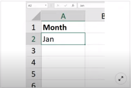
3. If you drag the fill handle (lower-right corner) of cell A2 downward into cells A3, A4 and A5, what contents will appear in those cells?

linkedin excel assessment test questions with answers

Jan, Jan, Jan
Feb, Mar, blank cell
Feb, Mar, Apr
FEB, MAR, APR

4. If cell A3 contains the text THE DEATH OF CHIVALRY, what will the function =PROPER(A3) return?

The death of chivalry
The Death of Chivalry
THE DEATH OF CHIVALRY
The Death Of Chivalry

5. In the worksheet below, you want to use data> subtotal to show a subtotal value per sport. What must do you BEFORE applying the subtotal function?

linkedin excel assessment test questions with answers

Format the data in column D
Sort by the data in column E
Sort by the data in column D
Format the data in column E

6. When editing a cell, what do you pass to cycle between relative, mixed and absolute cell references?

Alt+F4 (Windows) or Option+F4 (Mac)
Alt+Shift+4 (Windows) or Option+Shift+4 (Mac)
Ctrl+Shift+4 (Windows) or Command+Shift+4 (Mac)
the F4 key (Windows) or Command+T (Mac)

7. You need to add a line chart showing a sales trends over the last 12 months and you have only a little space to work with. How can you convey the required information within a single cell?

Add an image of the chart to a comment
Add a hyperlink to another worksheet that displays a chart when clicked
Add an image of the chart to the worksheet
Add a sparkline, a graphic that summarizes data visually within a single worksheet cell

8. What is the best way to activate the Excel Help system?

Right-click anywhere and select help
Press F1 or click the help tab in the ribbon
Press F10
All of these answers

9. Which format will display the value 27,500,000 as 27.5?

##,###,,
###.0,,
999.9,,
###,###.0,

10. When using Goal Seek, you can find a target result by varying___at most?

Three inputs
Four inputs
Two inputs
One input

11. In the image below, which option(s) can you select so that the appropriate field headers appear in cells A4 and B3 instead of the terms Row Labels and column Labels, respectively?

linkedin excel assessment test questions with answers

Show in Tabular Form
Show in Compact Form
Show in Compact Form or Show in Outline Form
Show in Tabular Form or Show in Outline Form

12. A cell contains the value 7.877 and you want it to display as 7.9 How can you accomplish this?

Use the ROUND( ) function.
Click the Decrease Decimal button twice.
Click the Decrease Decimal button once.
In the cells group on the home tab, click Format > Format cells. Then click the Alignment tab and select Right Indent.

13. Which formula is NOT equivalent to all of the others?

=A3+A4+A5+A6
=SUM(A3:A6)
=SUM(A3,A6)
=SUM(A3,A4,A5,A6)

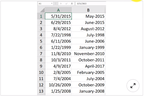
14. Which custom format will make the cells in column A appear like the corresponding cells in column B?

linkedin excel assessment test questions with answers

MMM-YYYY
MMMM-YYYY
MMMM&"-"&YYYY
M-YYYY

15. Which function returns a reference to a cell (or cell range) that is a specified distance from a base cell?

OFFSET
VLOOKUP
MATCH
INDEX

16. Which function returns the largest value in the range H2:H30?

=MAX(H2:H30)
=MAXIMUM(H2:H30)
=LARGE(H2:H30,29)
=UPPER(H2:H30,1)

17. Which chart type can display two different data series as different series types within the same chart?

XY chart
clustered column
bubble chart
combo chart

18. In the image below, what does clicking the button indicated by the green arrow do?

linkedin excel assessment test questions with answers

Hides or shows formula bar
Selects all
Hides or shows the ribbon
Selects objects

19. Which formula returns the value in cell A1 of the worksheet named MySheet?

=MySheet!A1
=MySheet_A1
=MySheet&A1
=MySheet@A1

20. In the worksheet below, you want to copy the formatting of cell A1 into cells B1:D1. Which approach (see arrows) accomplishes this the most efficiently?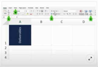
linkedin excel assessment test questions with answers

21. To round up a value to the nearest increment of your choice, such as the next five cents, what function should you use?

ROUNDUP
MAX
ROUND
CEILING

22. Which formula correctly counts the number of numeric values in both B4:E4 and G4:I4?

=COUNT(B4:E4&G4:I4)
=COUNT(B4:E4,G4:I4)
=COUNT(B4:E4 G4:I4)
=COUNT(B4:I4)

23. To ensure that a collection of shapes are evenly spaced apart from left to right, select the shapes, click page layout> Align, and then click___.

Align Center
Distribute Vertically
Align Middle
Distribute Horizontally

24. After activating a chart, which sequence adds a trendline to the chart?

In the Format group, select Trendline from the Insert Shapes list
Click outside the pilot area and select Add Trendline
Click inside the pilot area and select Forecast
Right-click a data series and select Add Trendline

25. Which Excel add-in will help you find a target result by varying multiple inputs to a formula?

Goal Seek
Data Analysis
Power Pivot
Solver

26. What tool would you use to prevent the input in a cell of a date outside a specific range?

Data Validation
Protect Workbook
Filter
Watch Window

27. What sequence allows you to print a worksheet with its top along the long edge of the paper?

1. Select Page Layout tab > Page Setup > Page

2. Under Orientation, click Portrait.

1. Click the Home tab

2. Click Orientation > Rotate Text Down

1. Click the Home tab

2. Click Orientation > Angle Clockwise

1. Select Page Layout tab > Page Setup > Page

2. Under Orientation, click Landscape

28. Your worksheet has the value 27 in cell B3. What value is returned by the function =MOD(B3,6)?

29. What tool would you use to prevent the input in a cell of a date outside a specific range?

Data Validation
Protect Workbook
Filter
Watch Window

30. Sheet1!C3 is the active cell. A new name is defined with the name Relative and with the reference Sheet1!A1. Cell E5 on Sheet1 is now selected.

What cell does Relative refer to?

A1
#NAME!
C3
E5

31. Cell A20 displays an orange background when its value is 5. Changing the value to 6 changes the background colour to green. What type of formatting is applied to cell A20?

cell style formatting
conditional formatting
tabular formatting
value formatting

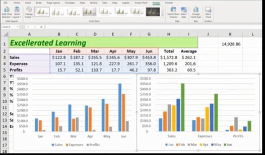
32. The charts below are based on the data in cells A3:G5. The chart on the right was created by copying the one on the left, Which ribbon button was clicked to change the layout of the chart on the right?
linkedin excel assessment test questions with answers

Quick Layout
Move Chart
Change Chart Type
Switch Row/Column

33. Which function returns TRUE if cell A1 contains a text value?

=ISTEXT(A1)
=ISALPHA(A1)
=ISCHAR(A11)
=ISSTRING(A1)

34. Which function returns the leftmost five characters in cell A1?

=A1.RIGHT(A1,LEN(A1).5)
=LEFT(A1,5)
=FIND(A1,1,5)
=SEARCH(A1,5)

35. When you format a range as a table, the filter buttons are applied by default. How can you turn off the button?

1.Select the table
2, Right-click anywhere in the table
3. Select Sort & Filter
4. Click the filter(funnel) icon

1.Select the header row
2, On the Home tab in the Editing section, select Sort & Filter
3. From the drop-down menu, select Turn Off Filter

1.Go to the Table Design tab
2. Select Sort & Filter
3. Click the filter(funnel) icon

1.Go to the Table Design tab
2, In the Table Style options, clear the Filter Button check box
3. Select Sort & Filter
4. Click the filter funnel icon

36. When you sort a list of numerical values into ascending or descending order, the value in the middle of the list is the ___.

mode
modulus
average
median

37. When the rightmost cell in the last column of an Excel table is the active cell, how do you create a new table row?

press the Tab key
press the Enter( Return) key
press the Esc key
press the Spacebar

38. What keystroke combination inserts a line break within a cell?

Ctrl+Shift+Enter (Windows) or Command+Shift+Return (Mac)
Alt+B (Windows) or Option+B (Mac)
Shift+Enter (Windows) or Shift+Return (Mac)
Alt+Enter (Windows) or Option+Return (Mac)

39. When importing XML data into a worksheet, Excel can interpret it by generating a ___if none is provided?

semantic map
data table
schema
lookup table

40. Excel has special formats for all of these kinds of numbers EXCEPT?

zip codes
telephone numbers
Social security numbers
Julian dates

41. Which statistical functions related to regression analysis ?

TREND and GROWTH
EXPONENTIAL and GROWTH
TREND and LINEAR
LINEAR and POLYNOMIAL

42. To insert a new column to the left of a specific column, right_click the header containing the column's letter and select___

Insert Column
Insert
Paste Special
Insert Column Left

43. How can you tell at a glance if any worksheets in the current workbook are grouped?

All of the grouped sheets are displayed on a single sheet tab
The word Group appears in the title bar at the top of the Excel screen
The word Group appears in the Status bar at the bottom of the Excel screen
The tabs on the worksheet flash in unison

44.What keystroke combination CANNOT be used as a shortcut to run a micro?

Ctrl+5
Ctrl+C
Ctrl+Shift+H
Ctrl+H

45. To unhide all hidden columns in a worksheet, select the entire worksheet and then do what?

Right-click a column header and select Reveal
Right-click a column header and select Unhide
Double-click a column header
Right-click a column header and select Column Width

46. In the worksheet shown, the cell range C2 :C7 contains formulas that return the PartClass value for each product. The PartClass starts at the fifth ProductSKU character (after KECO) and ends at the character before the Z- which will not always be the last character in the cell. What formula would you create in cell C2 (and copy to the other cell in the range) to return the PartClass number?

linkedin excel assessment test questions with answers

=MID(B2,5,MID("z",B2)-5)
=LEFT(B2,5,FIND("z",B2)-5)
=MID(B2,5,FIND("z",B2)-5)
=FIND(B2,5,MID("z",B2)-5)

47. You are working with columms whose witdth and font size should not be changed. Yet the columns are too narrow to display all the text in each cell. What tool should you use to solve this problem?

Sparklines
Wrap Text
Fill Handle
Centered Alignment

48. Of the four chart types listed, which works best for summarizing time-based data?

Pie chart
Line chart
XY scatter chart
Bar chart

49. The AutoSum formulas in the range C9:F9 below return unexpected values, Why is this?
linkedin excel assessment test questions with answers

The AutoSum formulas refer to the column to the left of their cells.
The AutoSum formulas exclude the bottom row of data.
The AutoSum formulas include the year at the top of each column in the calculation.
The AutoSum formulas include their own cells, creating a circular reference.

50. The text filter in column A is designed to display only those rows where the column A entry has a particular attribute. What is this attribute?

linkedin excel assessment test questions with answers

The second character in the cell is 9.
The number 9 appears one or more times within the cell.
The cell is comprised of 9 characters.
The number 9 appears once and only once within the cell.

51. An organization chart, which shows the hierarchy within a company or organization is available as____ that is included with excel?

a 3D model
SmartArt
a treemap chart
a drawing object

52. You want to be able to restrict values allowed in a cell and need to create a drop-down list of values from which users can choose. Which feature should you use?

Protect Worksheet
Conditional Formatting
Allows Users to Edit Ranges
Data Validation

53. You select cell A1 , hover the pointer over the cell border to raveal the move icon, then drug the cell to a new location. Which ribbon commands achieve the same result?

Copy and Paste
Cut and Fill
Copy and Transpose
Cut and Paste

54. Of the four chart types listed, which works best for summarizing time-based data?

Pie chart
Line chart
XY scatter chart
Bar chart

55. To discover how mainly cells in a range contain values that meet a single criterion. Use the ___ function?

SUMIFS
COUNTIF
COUNTA
COUNT

56. What is the term for an expression that is entered into a worksheet cell and begins with an equal sign?

contents
formula
function
argument

57. You want to add a column to the PrivotTable below that shows a 5% bonus for each sales rep. That data does not exist in the original data table. How can you do this without adding more data to the table?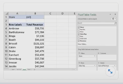
linkedin excel assessment test questions with answers

Add a new PrivotTable Field
Add a calculated field
Add a new summarize values by field
Add a calculated item

58. Review the worksheet below. Cell F2 needs a formula that uses INDEX and/or MATCH to display the product ID for the product name in cell E2 ("KS240 Panels")? What is the correct formula?
linkedin excel assessment test questions with answers

=INDEX(A2:A7,INDEX(E2,B2:B7,0))
=VLOOKUP(A2:A7,MATCH(E2,B2:B7,0))
=NATCH(A2:A7,INDEX(E2,B2:B7,0))
=INDEX(A2:A7,MATCH(E2,B2:B7,0))

59. What does this formula do?

=SUM(Sheet1 :Sheet4!D18)

It adds data from cell A1 of Sheet1 and cell D18 of Sheet4
It adds data from cell D18 of Sheet1 and cell D18 of Sheet4
It adds all data in the range A1:D18 in Sheet1, Sheet2, Sheet3 and Sheet4
It adds all data from all D18 cells in Sheet1, Sheet2, Sheet3 and Sheet4

60. How does the appearance of an array formula differ from that of a standard formula?

A heavy border appears around the range that is occupied by the array formula
When a cell that contains an array formula is selected , range finders appear on the worksheet arounds the formula's precedend cells.
In a worksheet cell, array formulas have a small blue triangle in the cells upper-right corner.
In the formula bar ,an array formula appears surrounded by curly brackets.

61. In a worksheet, column A contains employee last names , column B contains their middle initials(if any), and column C contains their first names, which tool can combine the last names, initials, and first names in column D without using a worksheet formula?

concatenation
Flash Fill
AutoFill
Columns to Text

𝓠4: How do I pass Linkedin Assessment in Excel?

Watch the video to see how I passed the Linkedin Excel Assessment test. The video can be helpful for those who are struggling with Linkedin Excel Assessment.

𝓠5: How do Linkedin assessments work?

The Linkedin assessment test is designed to determine the working efficiency of candidates. After taking any Linkedin Skill test, the Linkedin Authority will give you a report of the results.

If you pass, you will receive a badge that you can display on your profile if you wish. Badges are proof of your competency. Badges allow you to appear in the search list of employers that help you catch the eye of recruiters.

Closing Thoughts

Make sure you have acquired the necessary knowledge for the test. Refresh your skills once before taking an assessment test. Hope this was helpful for you.

Problem Solution